The standard way of using an RTD (resistance-temperature-detector) sensor is to include it in a bridge followed by a differential amplifier. The problem is that two nonlinearities – one from the sensor and another from the bridge – affect the transfer function. Some approaches are available that attempt to avoid the problem, but they tend to be bulky and expensive (reference 1, reference 2, and reference 3). An alternative circuit proposes adding only one extra resistor to the differential amplifier but provides neither design guidelines nor results (Reference 4). This Design Idea fills the gap. Although circuit analysis is somewhat complex, performance is good, and the circuit uses few components.
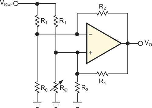
Besides the platinum RTD, Rθ, the circuit features only six precision resistors, an op amp, and a voltage reference (Figure 1). R4, the extra resistor for the differential amplifier, delivers additional current to the sensor that relates to the temperature you are measuring. With proper design, the circuit can provide good linearity and stability over a wide range of input temperatures. The output voltage, VO, depends on circuit components in the following way:

where YI = 1/RI and I = 0 to 4.
 |
|
| Figure 1 | This generic RTD circuit needs few components. |
For positive temperatures, a second-degree polynomial of the following form can approximate RTD characteristics:

where R0 is sensor resistance at 0 °C, α and β are coefficients, and Θ is the measured temperature.
After replacing the second equation in the first and doing some rearrangements, you get:

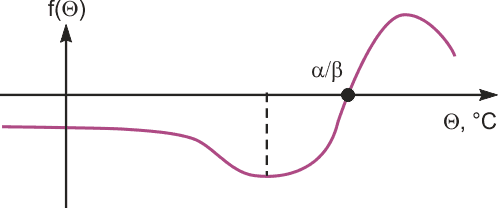
where B, C, and K are constants and f(Θ) is a function of temperature. Figure 2 shows the general shape of f(Θ). The output voltage depends linearly on temperature when f(Θ) is as close as possible to a constant. This situation is most true around the minimum point of f(Θ).
 |
|
| Figure 2 | The general shape of function f(Θ) varies with temperature. |
Some additional relations provide that the output voltage is 0 V at temperature 0 °C, the conversion coefficient is 10 mV/°C, the minimum of function f(Θ) is in the middle of the measurement span, and the current through RΘ causes negligible self-heating of the sensor.
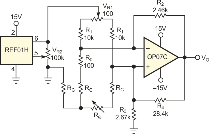
Figure 3 shows the circuit that meets these requirements. The sensor is a DIN-IEC 751 platinum RTD. Microsoft Excel software fits 13 points of 0 to 600 °C in steps of 50° from the RTD’s calibration table. The spreadsheet software determined R0 to have a value of 100 Ω, α to have a value of 3.908×10⁻³ °C–1, and β to have a value of –5.801×10⁻⁷ °C–2 with an R2 factor of one.
 |
|
| Figure 3 | The full circuit needs trimming potentiometers VR1 and VR2 to adjust zero and span, respectively, and a three-lead cable for sensor connection. RC is the cable’s resistance. |
All the circuit’s resistors have tolerances of 0.02%, and the temperature coefficient is 50 ppm/°C. You can use two trimming potentiometers, VR1 and VR2, to independently adjust zero and span readings. You should perform span adjustment at 550 °C to match the magnitudes of the positive and the negative errors. You can also extend the temperature range to start from –100 °C instead of 0 °C without exceeding the basic nonlinearity. The three-lead connection to the sensor significantly reduces the influence of connection-cable resistance, RC, on accuracy.
| Figure 1 | This generic RTD circuit needs few components. | ||||||||||||||||||
|
|||||||||||||||||||
Table 1 shows the results of evaluating this circuit’s performance with a calibrated, precision-decade resistance and a calibrated, 4.5-digit multimeter with readings at ambient temperatures of 24 and 68 °C; power supplies of ±12, ±15, and ±18 V; and cable resistances of 0 and 5 Ω.
References
- Bryant, James, Walt Jung, and Walter Kester, Op Amp Applications, Analog Devices, 2002.
- Villanucci, Robert S, “Design an RTD interface with a spreadsheet”
- Moghimi, Riza, “Low-error platinum RTD circuit has shutdown capability”
- Gutnikov, V.S., Integrated Electronics in Measuring Devices, Leningrad, 1980.
