Derek MacLachlan Staff Applications Engineer Keithley Instruments, Inc.
Accurate measurements are central to virtually every scientific and engineering discipline, but all too often measurement science gets little attention in the undergraduate curriculum. Even those who received a thorough grounding in measurement fundamentals as undergraduates can be forgiven if they’ve forgotten some of the details. This white paper is intended to refresh those fading memories or to bring those who want to learn more about making good quality measurements up to speed.
But what exactly does «good quality measurement» mean? Although it can mean a variety of things, one of the most important ones is the ability to create a test setup that’s suitable for the purpose intended. Let’s start with a typical test scenario that involves measuring some characteristics of a device or material. This can range from a very simple setup, such as using a benchtop digital multimeter (DMM) to measure resistance values, to more complex systems that involve fixturing, special cabling, etc. When determining the required performance of the system, that is, the required measurement accuracies, tolerances, speed, etc., one must include not only the performance of the measurement instrument but also the limitations imposed by and the effects of the cabling, connectors, test fixture, and even the environment under which tests will be carried out.
When considering a specific measurement instrument for an application, the specification or data sheet is the first place to look for information on its performance and how that will limit the results. However, data sheets are not always easy to interpret because they typically use specialized terminology.
Also, one can’t always determine if a piece of test equipment will meet the requirements of the application simply by looking at its specifications. For example, the characteristics of the material or device under test may have a significant impact on measurement quality. The cabling, switching hardware, and the test fixture, if required, can also affect the test results.
The Four-Step Measurement Process
The process of designing and characterizing the performance of any test setup can be broken down into a four-step process. Following this process will greatly increase the chances of building a system that meets requirements and eliminates unpleasant and expensive surprises.
Step 1
The first step, before specifying a piece of equipment, is to define the system’s required measurement performance. This is an essential prerequisite to designing, building, verifying, and ultimately using a test system that it will meet the application’s requirements. Defining the required level of performance involves understanding the specialized terminology like resolution, accuracy, repeatability, rise time, sensitivity, and many others.
Resolution is the smallest portion of the signal that can actually be observed. It is determined by the analog-to-digital (A/D) converter in the measurement device. There are several ways to characterize resolutionЧbits, digits, counts, etc. The more bits or digits there are, the greater the device’s resolution. The resolution of most benchtop instruments is specified in digits, such as a 6½-digit DMM. Be aware that the ½ digit terminology means that the most significant digit has less than a full range of 0 to 9. As a general rule, ½ digit implies the most significant digit can have the values 0, 1, or 2. In contrast, data acquisition boards are often specified by the number of bits their A/D converters have.
|
Although the terms sensitivity and accuracy are often considered synonymous, they do not mean the same thing. Sensitivity refers to the smallest change in the measurement that can be detected and is specified in units of the measured value, such as volts, ohms, amps, degrees, etc. The sensitivity of an instrument is equal to its lowest range divided by the resolution. Therefore, the sensitivity of a 16-bit A/D based on a 2 V scale is 2 divided by 65536 or 30 microvolts. A variety of instruments are optimized for making highly sensitive measurements, including nanovoltmeters, picoammeters, electrometers, and high-resolution DMMs. Here are some examples of how to calculate the sensitivity for A/Ds of varying levels of resolution:
- 3½ digits (2000) on 2 V range = 1 mV
- 4½ digits (20000) on 2-Omph range = 100 µOmph
- 16-bit (65536) A/D on 2 V range = 30 µV
- 8½ digits on 200 mV range = 1 nV
The implications of these terms are demonstrated by the challenge of ensuring the absolute accuracy of a temperature measurement of 100.00°C to ±0.01° versus measuring a change in temperature of 0.01°C. Measuring the change is far easier than ensuring absolute accuracy to this tolerance, and often, that is all that an application requires. For example, in product testing, it is often important to measure the heat rise accurately (for example, in a power supply), but it really doesn’t matter if it’s at exactly 25.00°C ambient.
Repeatability is the ability to measure the same input to the same value over and over again. Ideally, the repeatability of measurements should be better than the accuracy. If repeatability is high, and the sources of error are known and quantified, then high resolution and repeatable measurements are often acceptable for many applications. Such measurements may have high relative accuracy with low absolute accuracy.
Step 2
The next step gets into the actual process of designing the measurement system, including the selection of equipment and fixtures, etc. As mentioned previously, interpreting a data sheet to determine which specifications are relevant to a system can be daunting, so let’s look at some of the most important specs included:
 |
| Figure 1. |
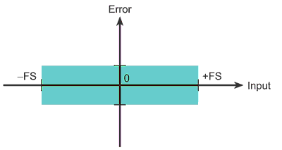
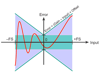
Accuracy. Keithley normally expresses its accuracy specifications in two parts, namely as a proportion of the value being measured, and a proportion of the scale that the measurement is on, for example: ± (gain error + offset error). This can be expressed as ± (% reading + % range) or ± (ppm of reading + ppm of range). The range in Figure 1 is represented by FS or «full scale.» For example, the specification for Keithley’s Model 2000 6.-digit multimeter, when measuring voltage on the 1 V range, states an accuracy of 30 ppm of the reading + 7ppm of range. The green box represents the offset error, which is expressed either as a percentage of the range or ppm of the range. Figure 2 illustrates the gain error, which is expressed either as a % of the reading or ppm of the reading. When carrying out a reading, we can expect the error to be anywhere within the purple and green areas of the graph. Accuracy specs for high-quality measurement devices can be given for 24 hours, 90 days, one year, two years, or even five years from the time of last calibration. Basic accuracy specs often assume usage within 90 days of calibration.
Temperature coefficient. Accuracy specs are normally guaranteed within a specific temperature range; for example, the Model 2000 DMM’s guaranteed range is 23 °C, ±5 °C. If carrying out measurements in an environment where temperatures are outside of this range, it’s necessary to add a temperature-related error. This becomes especially difficult if the ambient temperatures vary considerably.
Instrumentation error. Some measurement errors are a result of the instrument itself. As we have already discussed, instrument error or accuracy specifications always require two components: a proportion of the measured value, sometimes called gain error, and an offset value specified as a portion of full range. Let’s look at the different instrument specifications for measuring the same value. In this example, we are trying to measure 0.5 V on the 2 V range, using a lesser quality DMM. Using the specifications, we can see that the uncertainty, or accuracy, will be ± 350 µV. In abbreviated specs, frequently only the gain error is provided. The offset error, however, may be the most significant factor when measuring values at the low end of the range.
 |
| Figure 2. |
Accuracy = ±(% reading + % range) = ±(gain error + offset error)
For example, DMM 2V range:
Accuracy = ±(0.03% of reading + 0.01% range)
For a 0.5 V input:
Uncertainty = ±(0.03% . 0.5 V + 0.01% . 2.0 V = ±(0.00015 V + 0.00020 V) = ±350 µV
Reading = 0.49965 to 0.50035
In the next example, we have the same scenario, i.e., trying to measure 0.5 V using the 2 V range, but we are now using a better quality DMM. The example has better specifications on the 2 V range, and the uncertainty is now just ±35 µV.
DMM, 6½-digit, 2 V range (2.000000)
Accuracy = ±(0.003% reading + 0.001% range) =
= ±(30ppm readings + 10ppm range) = ±(0.003% reading + 20 counts)
Uncertainty 0.5 V = ±(0.000015 + 0.000020) = ±0.000035 V = ±35 µV
Now if we look at performing the same measurement using a data acquisition board, note that 1 LSB offset error is range/4096 = 0.024% of range. On a 2 V range, 1 LSB offset error is 0.488 millivolt. Note that the measurement accuracy is much poorer with this data acquisition card than when using the higher quality benchtop DMM.
Analog input board, 12 bit, 2V range
Accuracy = ±(0.01% reading + 1 LSB) = ±(100 ppm + 1 bit)
Uncertainty 0.5 V = ±(0.000050 + 2.0/4096) = ±(0.000050 + 0.000488) = ±0.000538 = ±538 µV
Sensitivity. Sensitivity, the smallest observable change that can be detected by the instrument, may be limited either by noise or by the instrument’s digital resolution. The level of instrument noise is often specified as a peak-to-peak or RMS value, sometimes within a certain bandwidth. It is important that the sensitivity figures from the data sheet will meet your requirements, but also consider the noise figures as these will especially affect low level measurements.
Timing. What does the timing within a test setup mean? Obviously, an automated PC-controlled measurement setup allows making measurements far more quickly than manual testing. This is especially useful in a manufacturing environment, or where many measurements are required. However, it’s critical to ensure that measurements are taken when the equipment has «settled» because there is always a tradeoff between the speed with which a measurement is made and its quality. The rise time of an analog instrument (or analog output) is generally defined as the time necessary for the output to rise from 10% to 90% of the final value when the input signal rises instantaneously from zero to some fixed value. Rise time affects the accuracy of the measurement when it’s of the same order of magnitude as the period of the measurement. If the length of time allowed before taking the reading is equal to the rise time, an error of approximately 10% will result, because the signal will have reached only 90% of its final value. To reduce the error, more time must be allowed. To reduce the error to 1%, about two rise times must be allowed, while reducing the error to 0.1% would require roughly three rise times (or nearly seven time constants).